Loading the data

There are three datafiles we have out of the measurements. Let’s load them all into memory with read_photons function:

tt = photonscore.read_photons('tirf.photons');
wf = photonscore.read_photons('wf.photons');
rwf = photonscore.read_photons('irf_wf.photons');

% get time channel width in ps.
dt_channel = photonscore.file_info('tirf.photons').dt_channel;

For example, "tirf.photons" dataset:

>> tt

tt =

  struct with fields:

     x: [79339363×1 uint16]
     y: [79339363×1 uint16]
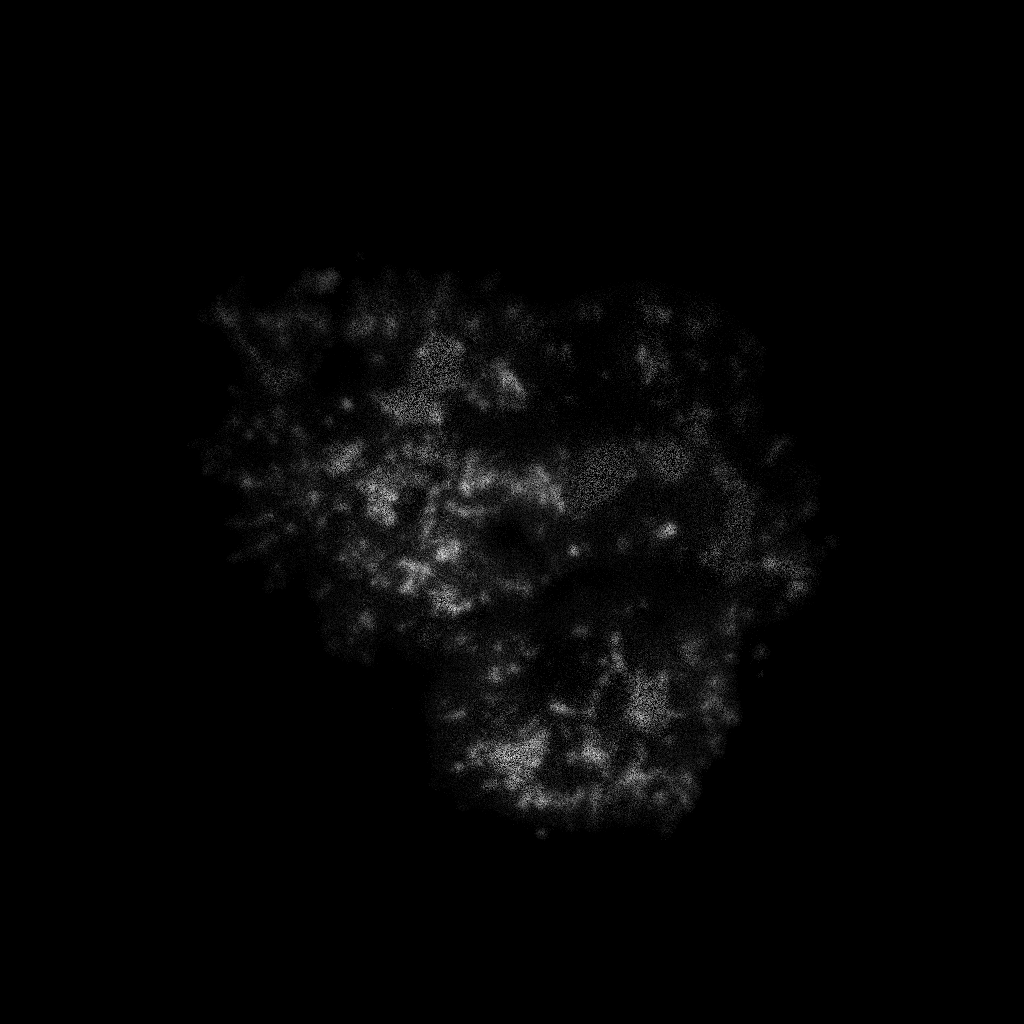
    dt: [79339363×1 uint16]

Take a look at the images

Here for hist_2d call we use the binning range from 0 to 4096 that is the whole range of the recorded positions and we specify 1024 as a number of bins in this range.

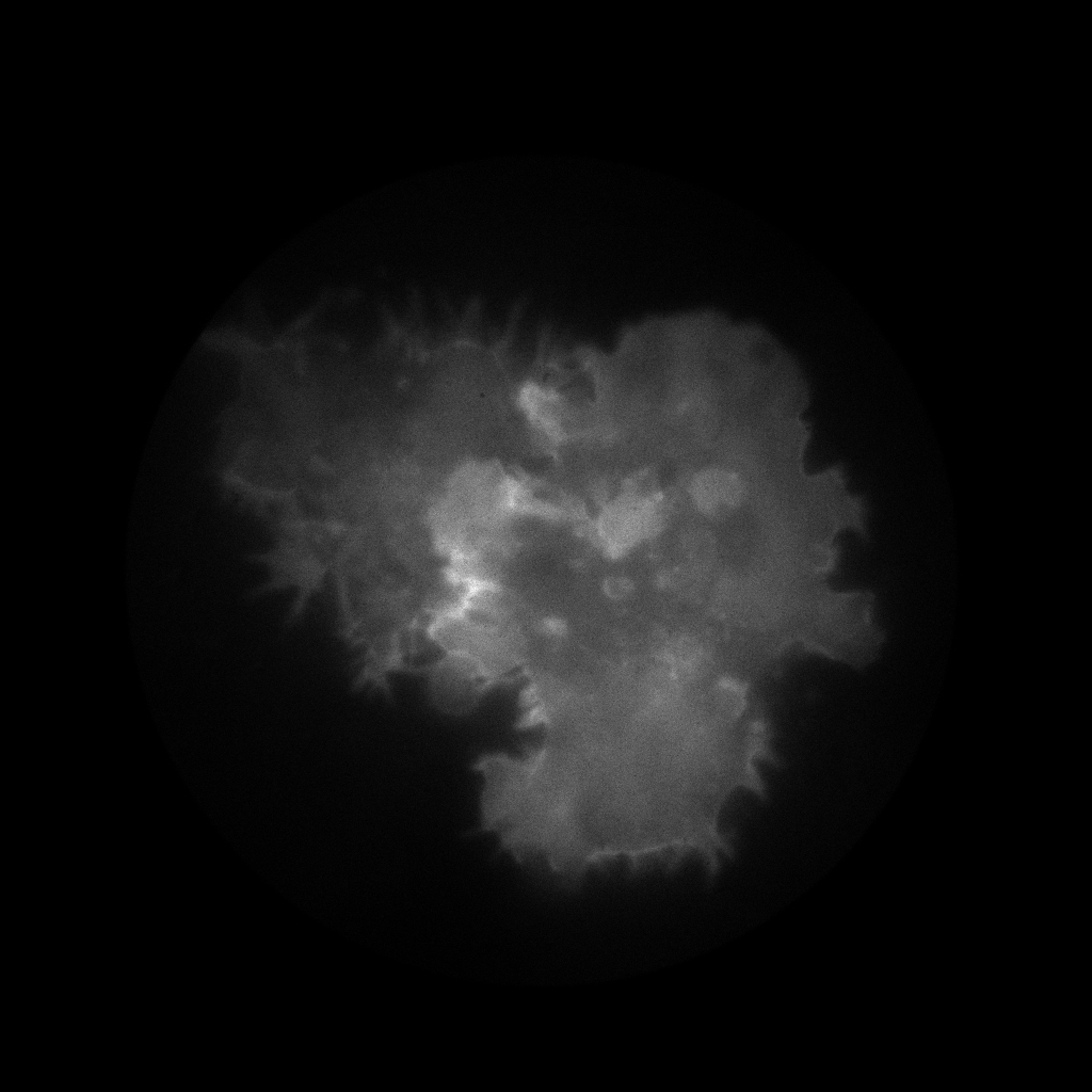
As we can see on the figure there is enough photons to go with 1 “megapixel” binning. Ok, lets sort the data with flim.sort function fixing the binning size:

fl_tt = photonscore.flim.sort(tt.x, 0, 4096, 1024, tt.y, tt.dt);
fl_wf = photonscore.flim.sort(wf.x, 0, 4096, 1024, wf.y, wf.dt);
fl_rwf = photonscore.flim.sort(rwf.x, 0, 4096, 1024, rwf.y, rwf.dt);

The sorting routine is a compute-intense operation. The duration may vary depending on CPU speed and number of cores in the system. Once the data sorting is done, one can compute mean and median lifetimes:

[md_tt, me_tt] = photonscore.flim.medimean(fl_tt);
[md_wf, me_wf] = photonscore.flim.medimean(fl_tt);

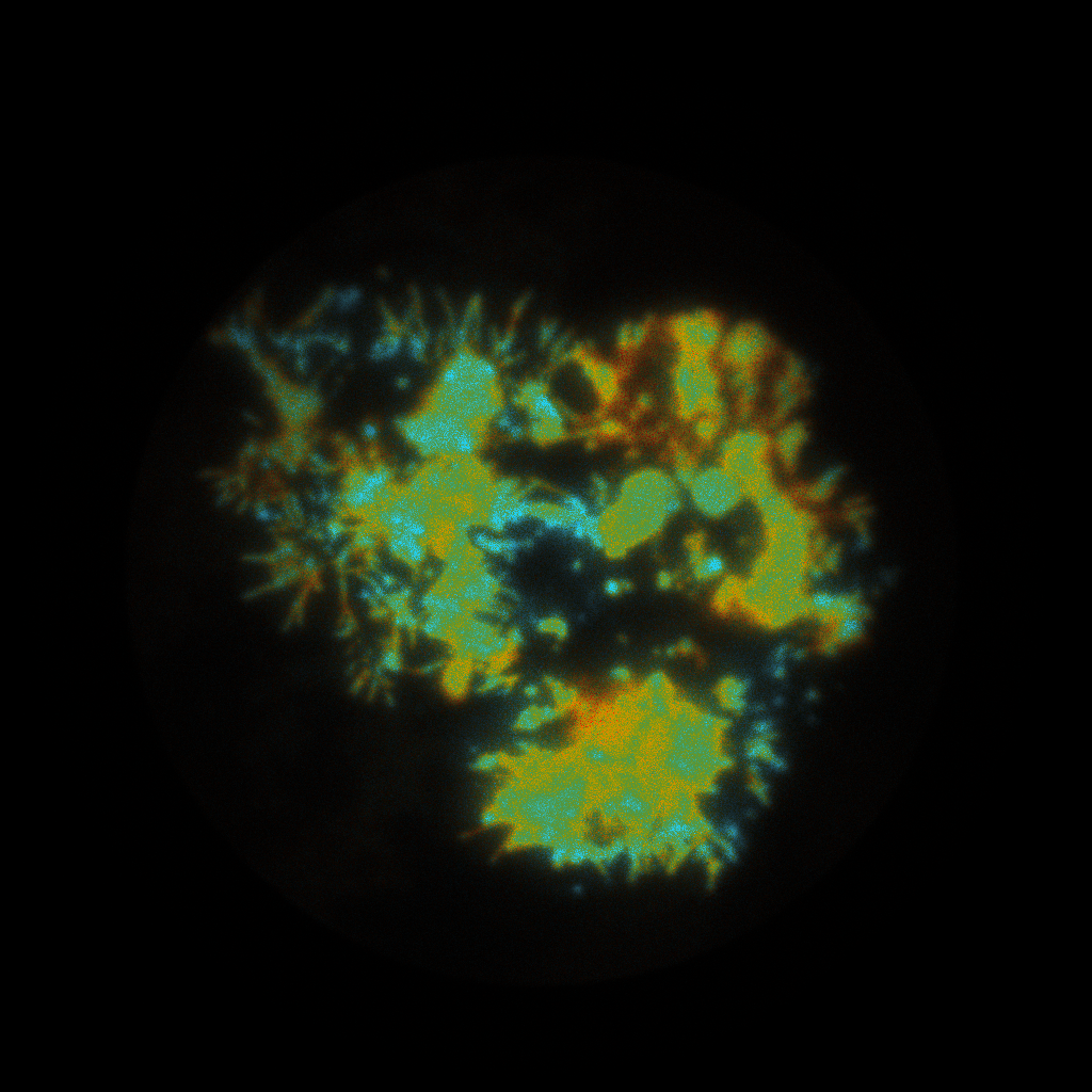
Here we use flim.iw_tau to visualize intensity weighted median (or mean me_tt and me_wf) lifetimes:

subplot(1,2,1)
img_tt = photonscore.flim.iw_tau(fl_tt.image, md_tt);
imagesc(img_tt);
pbaspect([1 1 1]);

subplot(1,2,2)
img_wf = photonscore.flim.iw_tau(fl_wf.image, md_wf);
imagesc(img_wf);
pbaspect([1 1 1]);

The resulting intensity-weighted lifetime images with a default preview.png palette applied:

Fitting the lifetimes

First, let us to take a look on the decays:

r = [0 4095];
h_tt = photonscore.hist_1d(fl_tt.time, r(1), r(2), r(2)-r(1));
h_wf = photonscore.hist_1d(fl_wf.time, r(1), r(2), r(2)-r(1));
h_rwf = photonscore.hist_1d(fl_rwf.time, r(1), r(2), r(2)-r(1));

x = (r(1):r(2)-1);

figure('Position', [0 0 1000 500])
semilogy(x, h_tt);
hold on;
semilogy(x, h_wf);
semilogy(x, h_rwf);
hold off;
legend 'TIRF' 'Wide-field' 'IRF'
xlabel 'Time [channel]'
ylabel 'Counts'

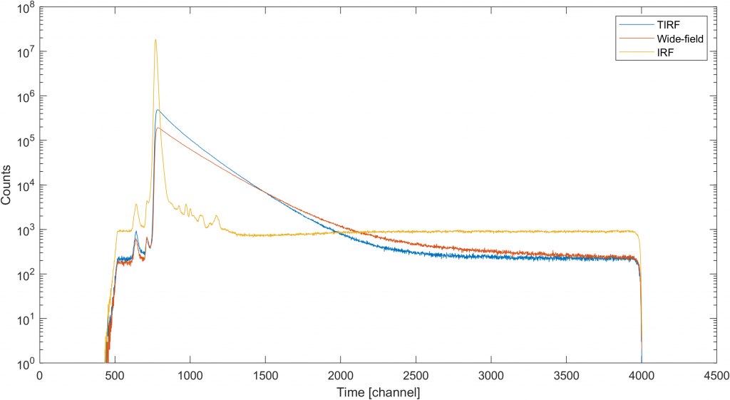
The result of the above code should look similar to figure below where we can see the whole of our timing signal. Obviously, one would not need everything from the range acquired. So, the first thing we redefine the range changing the first line in the fragment above to r = [550 3930]; to focus only on the sub-range of the time window.

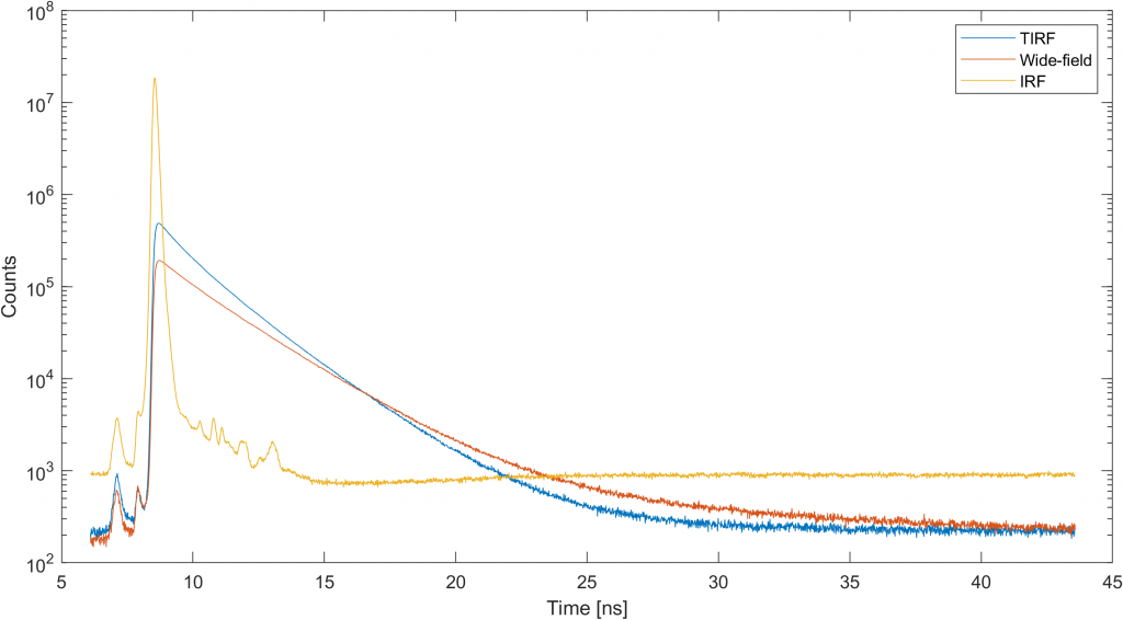
The second observation one shall do is IRF background that should be removed by subtracting 950 from the histogram. Let us introduce variable h_rwf_nbg that holds background-free IRF and proceed with discrete fitting:

h_rwf_nbg = max(0, h_rwf - 950);
[x1att, m1att] = photonscore.flim.fit_decay_auto(h_rwf_nbg, h_tt, 4);
photonscore.flim.plot_fit_decay_model(m1att, h_rwf_nbg, h_tt, dt_channel);

The purpose of the discrete fit isto find irf_shift and tau_ref parameters to proceed with MEM analysis:

>> x1att

x1att = 

  struct with fields:

     irf_shift: -0.1993
       tau_ref: 2.3187
    background: 236.0657
             a: [4×1 double]
           tau: [4×1 double]
    likelihood: 9.3256e+03

In this particular dataset the shift parameter is close to zero (-0.1993). But the reference dye lifetime (2.3187 or 25.7 ps) will be very helpful for further analysis:

% generate exponentially spaced tau
tau = photonscore.flim.log_tau_range(400, [10 800]);

% Create a model for admixture expectation maximization routine
m = photonscore.flim.convolve(...
    h_rwf_nbg/sum(h_rwf_nbg), ... % with normalized to 1 IRF
    x1tt.irf_shift,... % IRF shift we got with discrete fit
    length(h_tt), ... % number of time channels
    tau,...
    x1tt.tau_ref); % use delta function reconvolution

% append background component
m = [m ones(size(m,1), 1)/size(m,1)];

[x2tt m2tt] = photonscore.flim.admixture_em(m, h_tt, ones(size(m,2), 1), ...
    'iterations', 20000);

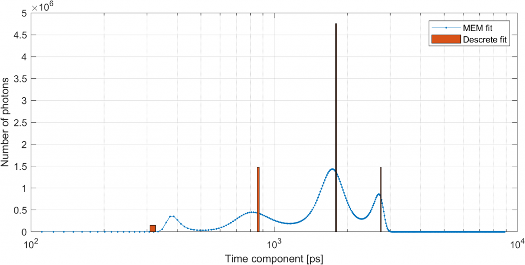
Using the lifetimes obtained here we can proceed with a per pixel fit.

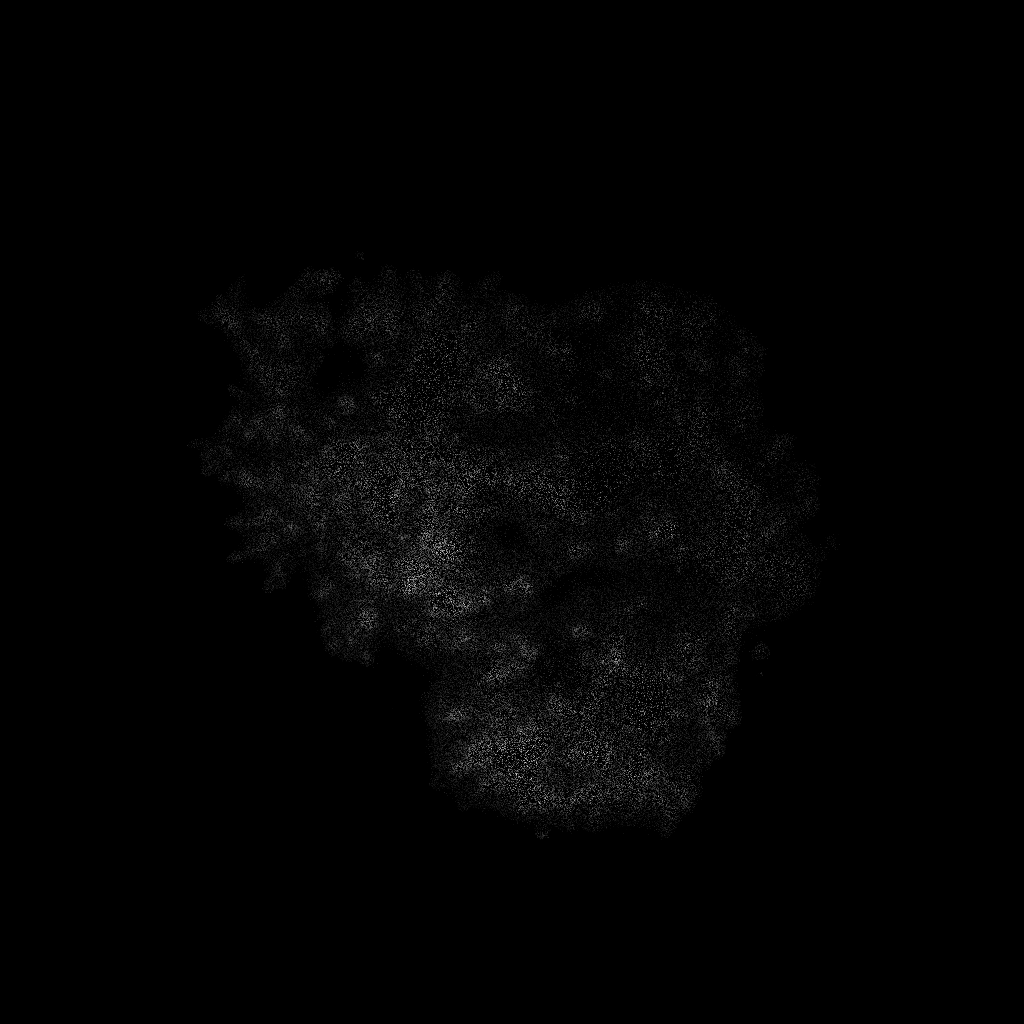
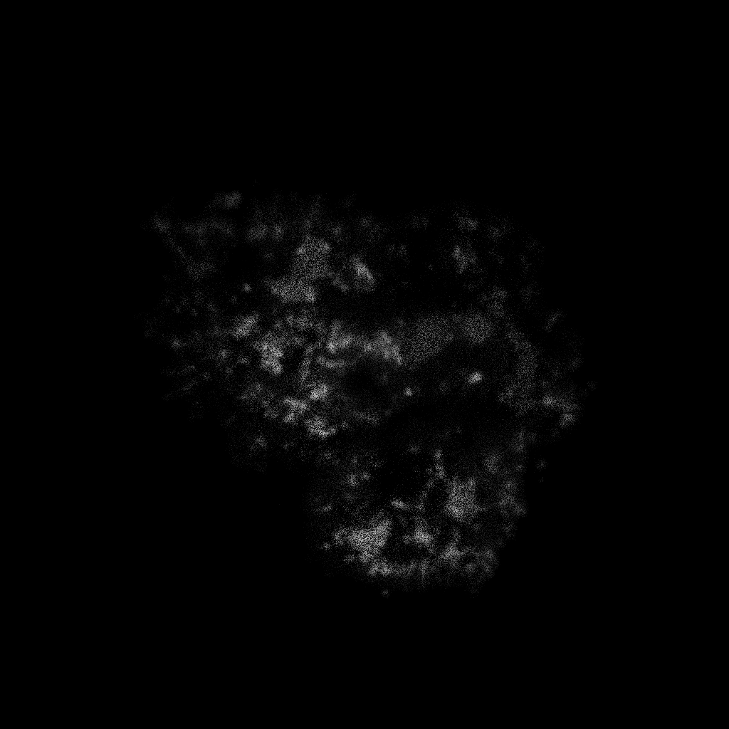
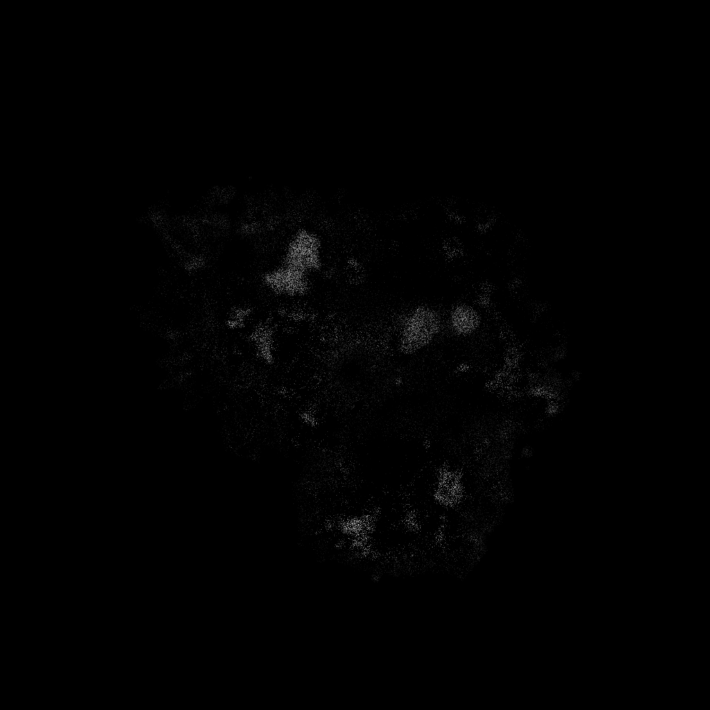
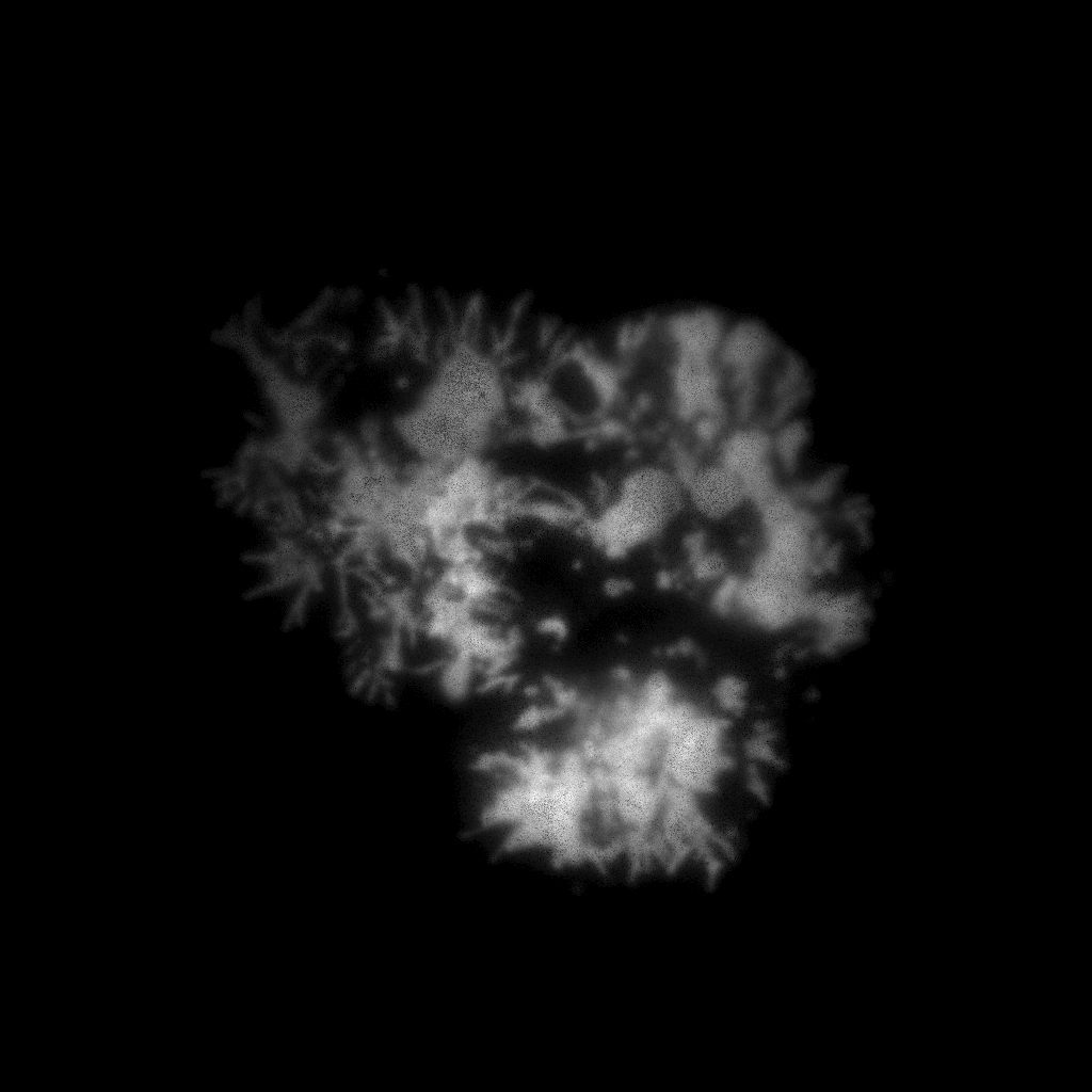
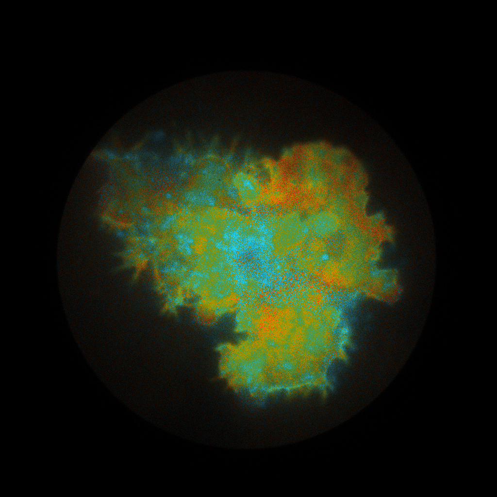
Results

The main results are depicted below. The images show “fast” fraction and “slow” fraction of the admixture resolving analysis. The “fast” components relate to the molecules those are closer to the metal covered surface than the rest: